
The Earth's Magnetic Field: An Overview
Contents
- 1 Introduction
- 2 Geomagnetic field observations
- 2.1 Definitions
- 2.2 Observatories
- 2.3 Satellites
- 2.4 Other direct observations
- 2.5 Indirect observations
- 3 Characteristics of the Earth's magnetic field
- 3.1 Reversals
- 3.2 The present magnetic field
- 3.3 Westward drift
- 3.4 Geomagnetic jerks
- 3.5 Crustal magnetic field
- 3.6 Field variations at quiet times
- 3.7 Field variations at disturbed times
- 4 The Earth's magnetic field as both a tool and a hazard in the modern world
- 4.1 Navigation
- 4.2 Directional drilling
- 4.3 Geomagnetically induced currents
- 4.4 Satellite operations
- 4.5 Exploration geophysics
- Bibliography
1 Introduction
The Earth's magnetic field is generated in the fluid outer core by a self-exciting dynamo process. Electrical currents flowing in the slowly moving molten iron generate the magnetic field. In addition to sources in the Earth's core the magnetic field observable at the Earth's surface has sources in the crust and in the ionosphere and magnetosphere. The geomagnetic field varies on a range of scales and a description of these variations is now made, in the order low frequency to high frequency variations, in both the space and time domains. The final section describes how the Earth's magnetic field can be both a tool and a hazard to the modern world. First of all, however, methods of observing the magnetic field are described.
Back to the top of the page
2 Geomagnetic field observations
2.1 Definitions
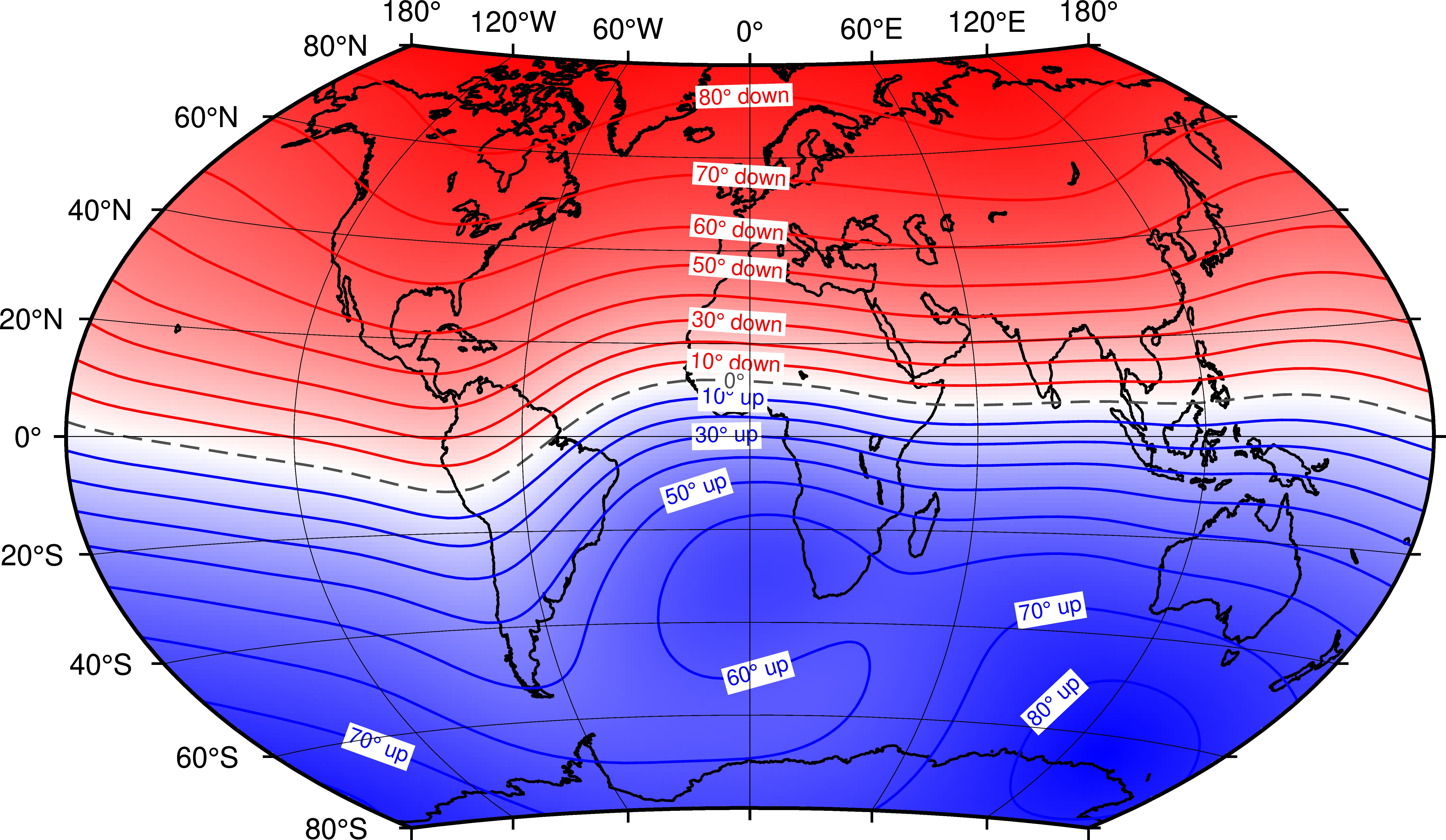
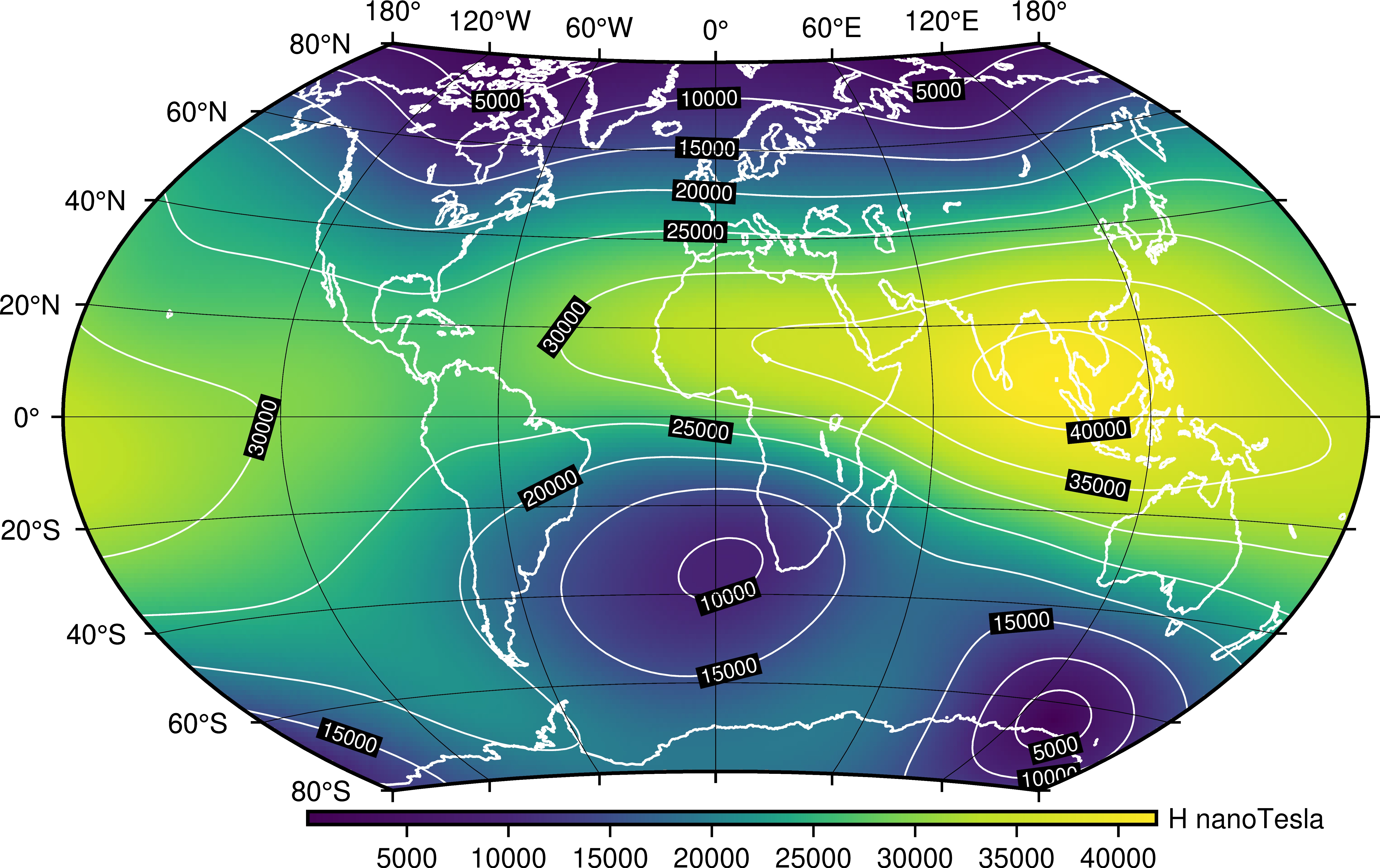
The geomagnetic field vector, B, is described by the orthogonal components X (northerly intensity), Y (easterly intensity) and Z (vertical intensity, positive downwards); total intensity F; horizontal intensity H; inclination (or dip) I (the angle between the horizontal plane and the field vector, measured positive downwards) and declination (or magnetic variation) D (the horizontal angle between true north and the field vector, measured positive eastwards). Declination, inclination and total intensity can be computed from the orthogonal components using the equations
where H is given by
 .
.
The International System of Units (SI) unit of magnetic field intensity, strictly flux density, most commonly used in geomagnetism is the Tesla. At the Earth's surface the total intensity varies from 22,000 nanotesla (nT) to 67,000 nT. Other units likely to be encountered are the Gauss (1 Gauss = 100,000 nT), the gamma (1 gamma = 1 nT) and the �rsted.
Back to the top of the page
2.2 Observatories
A geomagnetic observatory is a location where absolute vector observations of the Earth's magnetic field are recorded accurately and continuously, with a time resolution of one minute or less, over a long period of time. The site of the observatory must be magnetically clean and remain so for the foreseeable future. The earliest magnetic observatories where continuous vector observations were made began operation in the 1840s.
There are two main categories of instruments at an observatory. The first category comprises variometers which make continuous measurements of elements of the geomagnetic field vector but in arbitrary units, for example millimetres of photographic paper in the case of photographic systems or electrical voltage in the case of fluxgates. A fluxgate sensor comprises a core of easily saturable material with high permeability. Around the core there are two windings: an excitation coil and a pick-up coil. If an alternating current is fed into the excitation coil so that saturation occurs and if there is a component of the external magnetic field along the fluxgate element, the pick-up coil outputs a signal not only with the excitation frequency but also other harmonics related to the intensity of the external field component. Both analogue and digital variometers require temperature-controlled environments and installation on extremely stable platforms (though some modern systems are suspended and therefore compensate for platform tilt). Even with these precautions they can still be subject to drift. They operate with minimal manual intervention and the resulting data are not absolute.
The second category comprises absolute instruments which can make measurements of the magnetic field in terms of absolute physical basic units or universal physical constants. The most common types of absolute instrument are the fluxgate theodolite for measuring D and I and the proton precession magnetometer for measuring F. In the former the basic unit is an angle. The fluxgate sensor mounted on the telescope of a non-magnetic theodolite is used to detect when it is perpendicular to the magnetic field vector. Collimation errors between the fluxgate sensor and the optical axis of the theodolite and within the theodolite are minimised by taking readings from four telescope positions. With the fluxgate sensor operating in null-field mode the stability and sensitivity of the sensor and its electronics are maximised. True north is determined by reference to a fixed mark of known azimuth. This can be determined astronomically or by using a gyro attachment. In a proton precession magnetometer the universal physical constant is the gyromagnetic ratio of the proton and the basic unit is time (frequency). Measurements with a fluxgate theodolite can only be made manually whilst a proton magnetometer can operate automatically.
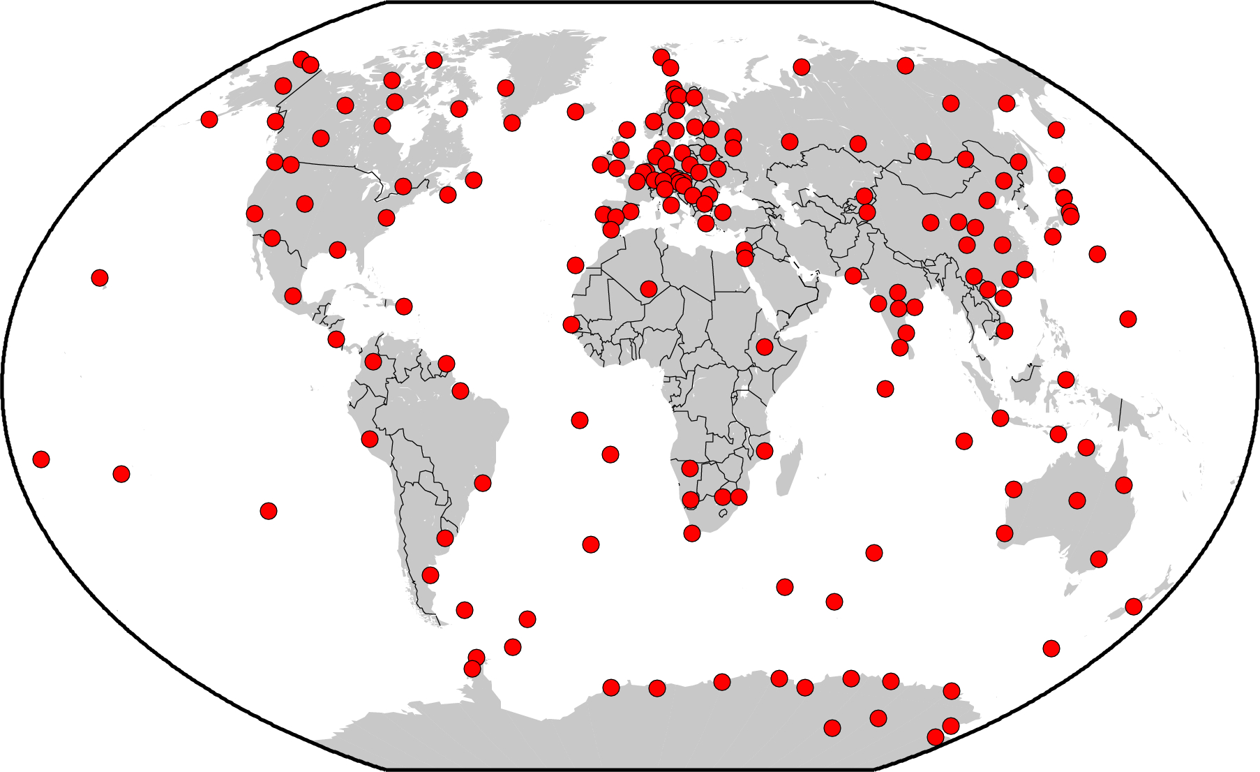
The locations of currently operating magnetic observatories are shown in Figure 1. It can be seen that the spatial distribution of the observatories is rather uneven, with a concentration in Europe and a dearth elsewhere in the world, particularly in the ocean areas.
Back to the top of the page
2.3 Satellites
Since the 1960s the Earth's magnetic field has been observed intermittently by satellites. The first satellites measured only the strength of the magnetic field, sometimes using only a non-absolute instrument, but latterly there have been a number of satellite missions measuring the full field vector, using star cameras to establish the direction of a triaxial fluxgate sensor. An absolute intensity instrument is normally also carried and both magnetic instruments are kept remote from the main body of the satellite by mounting them at the end of a non-magnetic boom. Satellites provide an excellent global distribution of data but generally only last for a short period of time, i.e. months to a few years.
Satellites which have provided/are providing valuable vector data for geomagnetic field modelling are Magsat, which flew in 1979 and 1980, �rsted and CHAMP which were launched in 1999 and 2000 respectively, and Swarm, launched in 2013. Ørsted returned vector data till 2006 and thereafter continued to return scalar data till 2013. CHAMP re-entered the Earth's atmosphere in September 2010 after more than 10 years of collecting vector magnetic data. The Swarm mission comprises 3 identical satellites. The �rsted satellite took over 2 years to sample all local times and flew in the altitude range 640-850 km. The CHAMP satellite sampled all local times in 4-5 months and flew in the altitude range 330-450 km. Two of the Swarm satellites fly side by side at altitudes (late 2014) of about 470 km and the third is at an altitude of about 520 km. The sampling rate of local times between the lower and upper satellites differs slightly. The lower two satellites are intended for very fine resolution of the magnetic field generated by the rocks in the Earth's crust. The upper satellite provides a simultaneous measurement at a different location. This is important for identifying magnetic fields generated by the magnetosphere and ionosphere.
Back to the top of the page
2.4 Other direct observations
The Earth's magnetic field is observed in a number of other ways. These are repeat stations and surveys made on land, from aircraft and ships. Repeat stations are permanently marked sites where high-quality vector observations of the Earth's magnetic field are made for a few hours, sometimes a few days, every few years. Their main purpose is to track changes in the core-generated magnetic field.
Most aeromagnetic surveys are designed to map the crustal field. As a result they are flown at altitudes lower than 300 m, they cover small areas, generally once only, with very high spatial resolution. Because of the difficulty in making accurately oriented measurements of the magnetic field on a moving platform, these kinds of aeromagnetic surveys generally comprise total intensity data only. However, between 1953 and 1994 the Project MAGNET programme collected high-level three-component aeromagnetic data specifically for modelling the core-generated field. The surveys were mainly over the ocean areas of the Earth, at mid to low latitudes. A variety of platforms and instrumentation were used; the most recent set-up included a fluxgate vector magnetometer mounted on a rigid beam in the magnetically clean rear part of the aircraft, a ring laser gyro fixed at the other end of the beam, and a scalar magnetometer located in a stinger extending some distance behind the aircraft's tail section.
Modern marine magnetic surveys are also invariably designed to map the crustal field but with careful processing it is possible to obtain information about the core-generated field from the data. In a marine magnetic survey a scalar magnetometer is towed some distance behind a ship, usually along with other geophysical equipment, as it makes either a systematic survey of an area or traverses an ocean.
Magnetic observations prior to the establishment of observatories and an absolute method of measuring magnetic intensity by Gauss in the 1830s were made, amongst others, by mariners engaged in merchant and naval shipping. These are mainly of declination and extend the global historic dataset back to the beginning of the 17th century.
Back to the top of the page
2.5 Indirect observations
Prior to the 17th century indirect observations of the Earth's magnetic field are possible from archaeological remains and rocks using palaeomagnetic techniques. The subject of rock magnetism and palaeomagnetism is outwith the scope of this article.
Back to the top of the page
3 Characteristics of the Earth's magnetic field
3.1 Reversals
When a rock is formed it usually acquires a magnetisation parallel to the ambient magnetic field, i.e. the core-generated field. From careful analyses of directions and intensities of rock magnetisation from many sites around the world it has been established that the polarity of the axial dipole has changed many times in the past, with each polarity interval lasting several thousand years. These reversals occur slowly and irregularly, and for a period of about 30 million years around about 100 million years before present, there were no reversals at all. In addition to full reversals there have been many aborted reversals when the magnetic poles are observed to move equatorwards for a while but then move back and align closely with the Earth's spin axis. The solid inner metal core is thought to play an important role in inhibiting reversals. At the present time we are seeing a 6% decline in the dipole moment per century. Whether this is a sign of an imminent reversal is difficult to say.
Back to the top of the page
3.2 The present magnetic field
In a source-free region near the surface of the Earth the magnetic field is the negative gradient of a scalar potential which satisfies Laplace's equation. A solution to Laplace's equation in spherical coordinates is called a spherical harmonic expansion and its parameters are called Gauss coefficients. There are internal or external coefficients, modelling the field generated inside or outside the Earth respectively. A separation of the core and crustal fields, both internal, is not perfect. The internal field is often called the main field.
The main-field coefficients change with time as the core-generated field changes, and in commonly used spherical harmonic models, for example the International Geomagnetic Reference Field (IGRF) and the World Magnetic Model, this secular variation is assumed to be constant over 5-year intervals. It has only been possible to accurately determine the small but persistent field generated outside the Earth, largely by the ring current, since satellite data have become available.
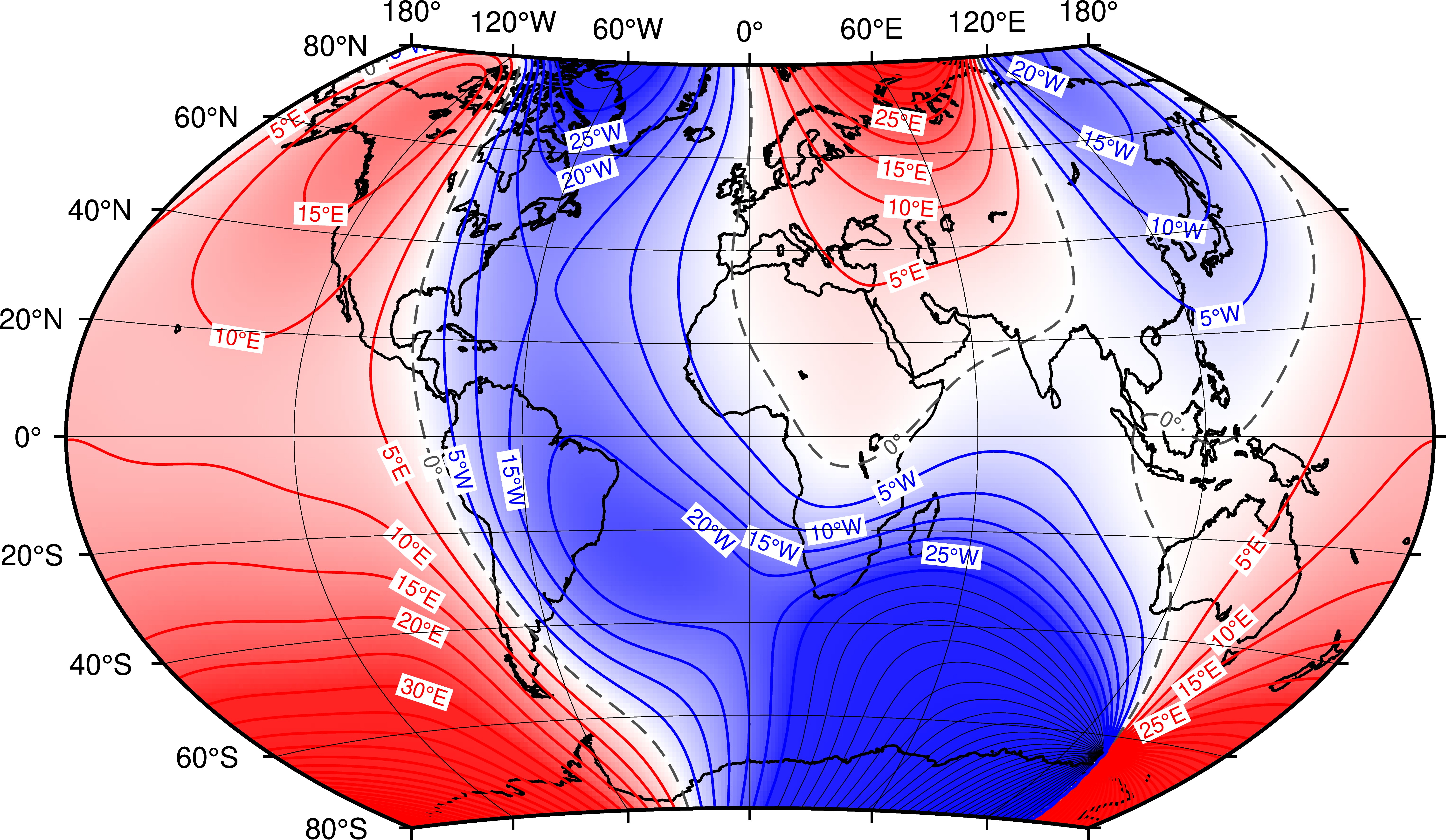
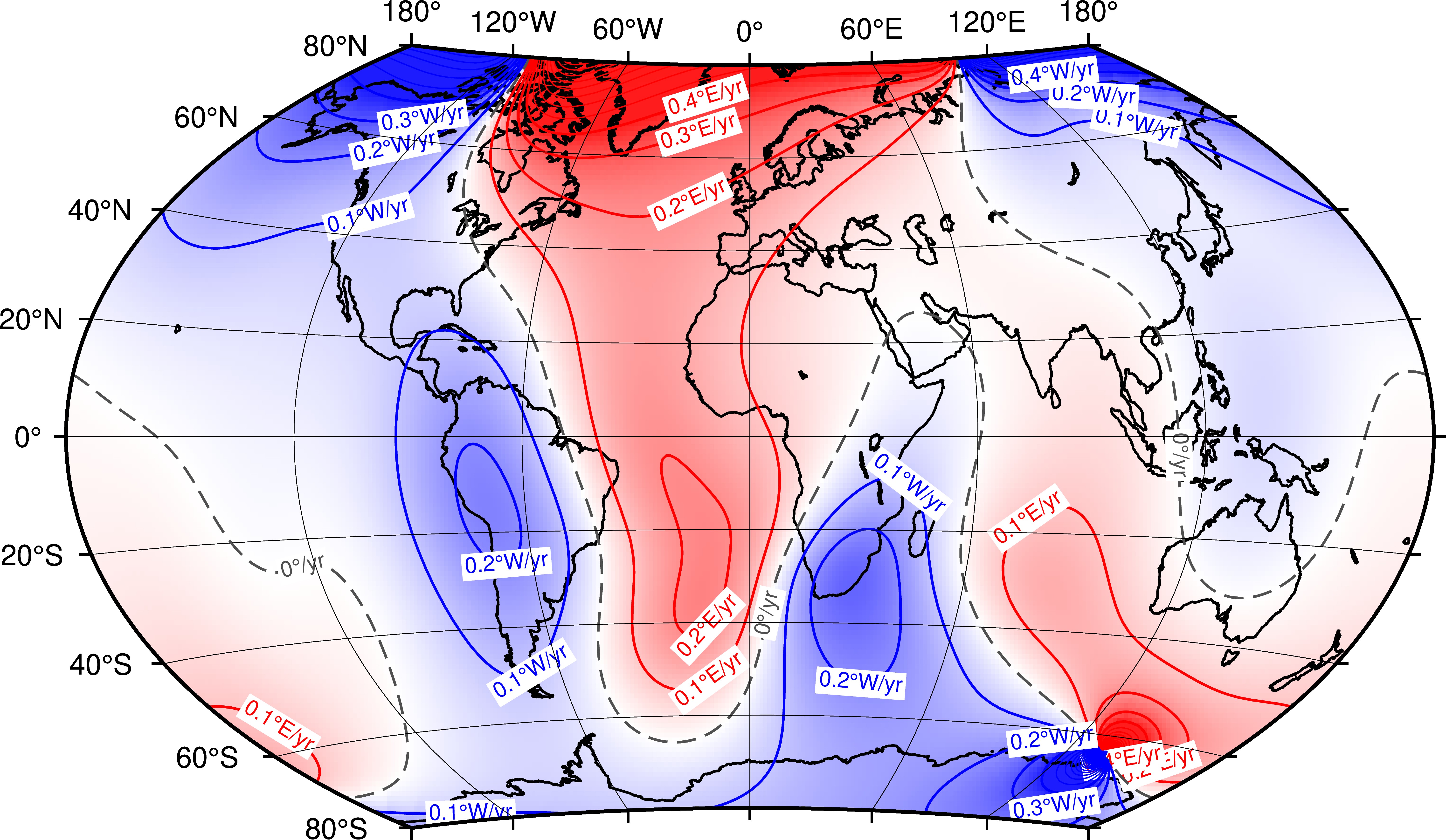
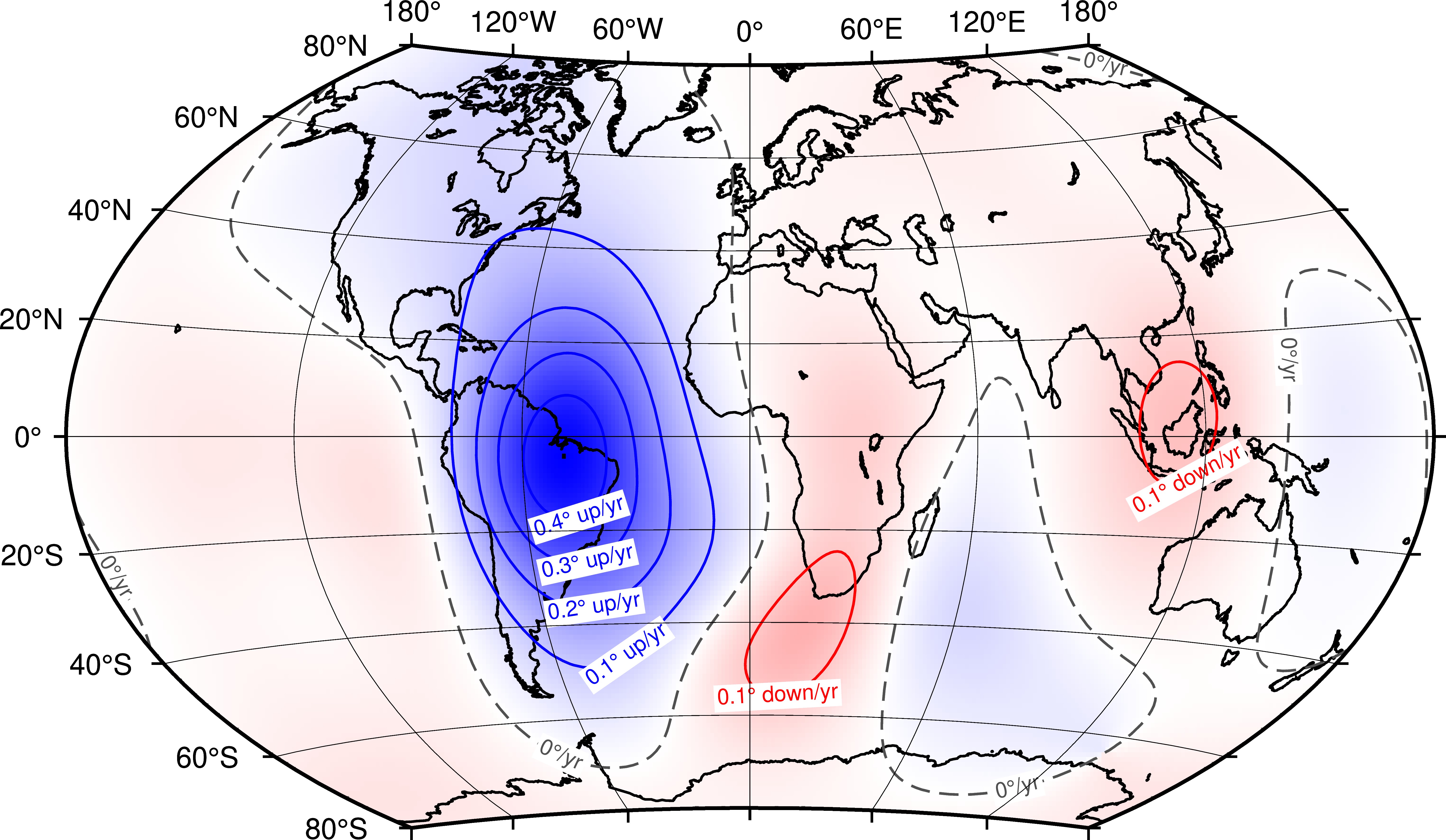
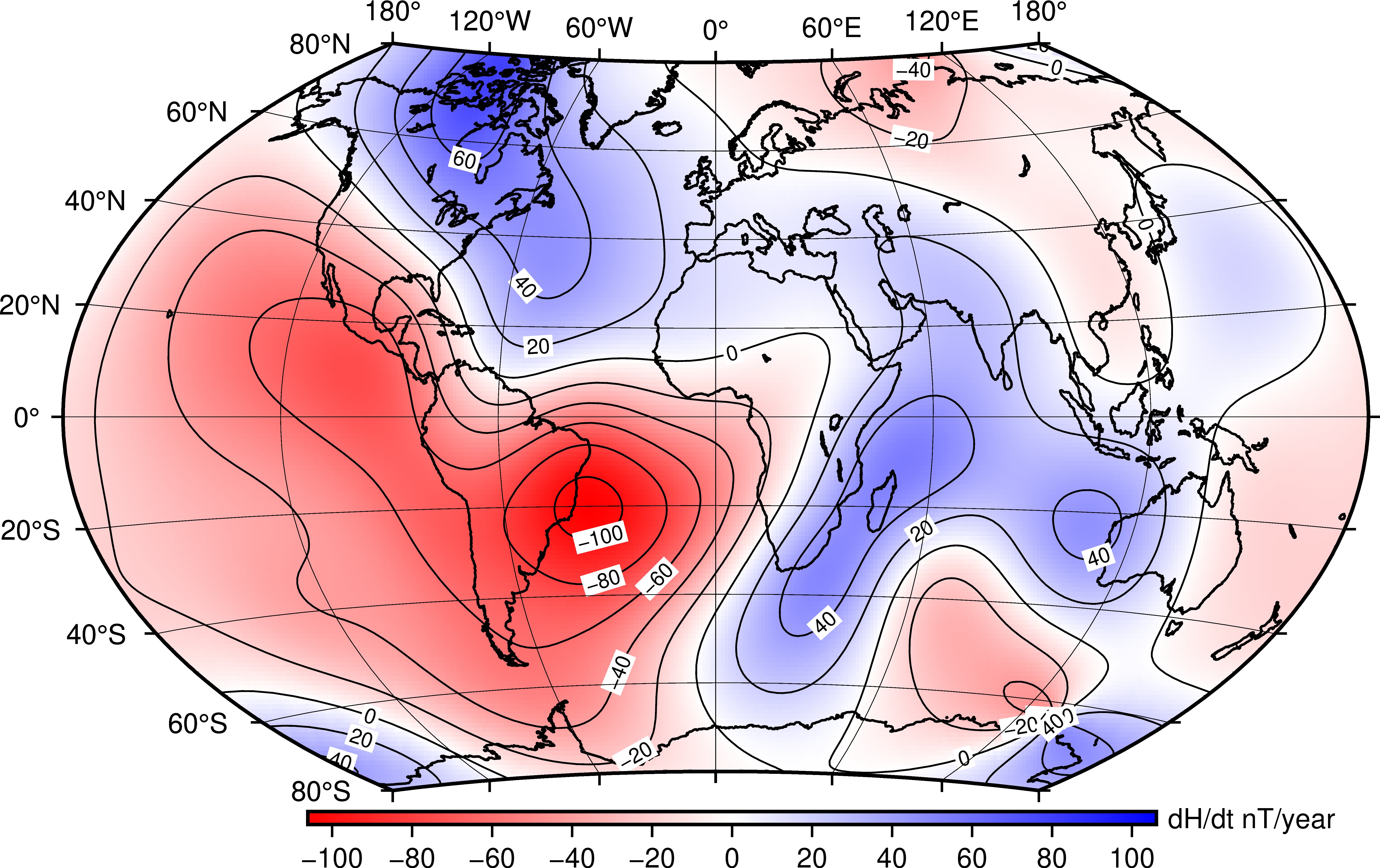
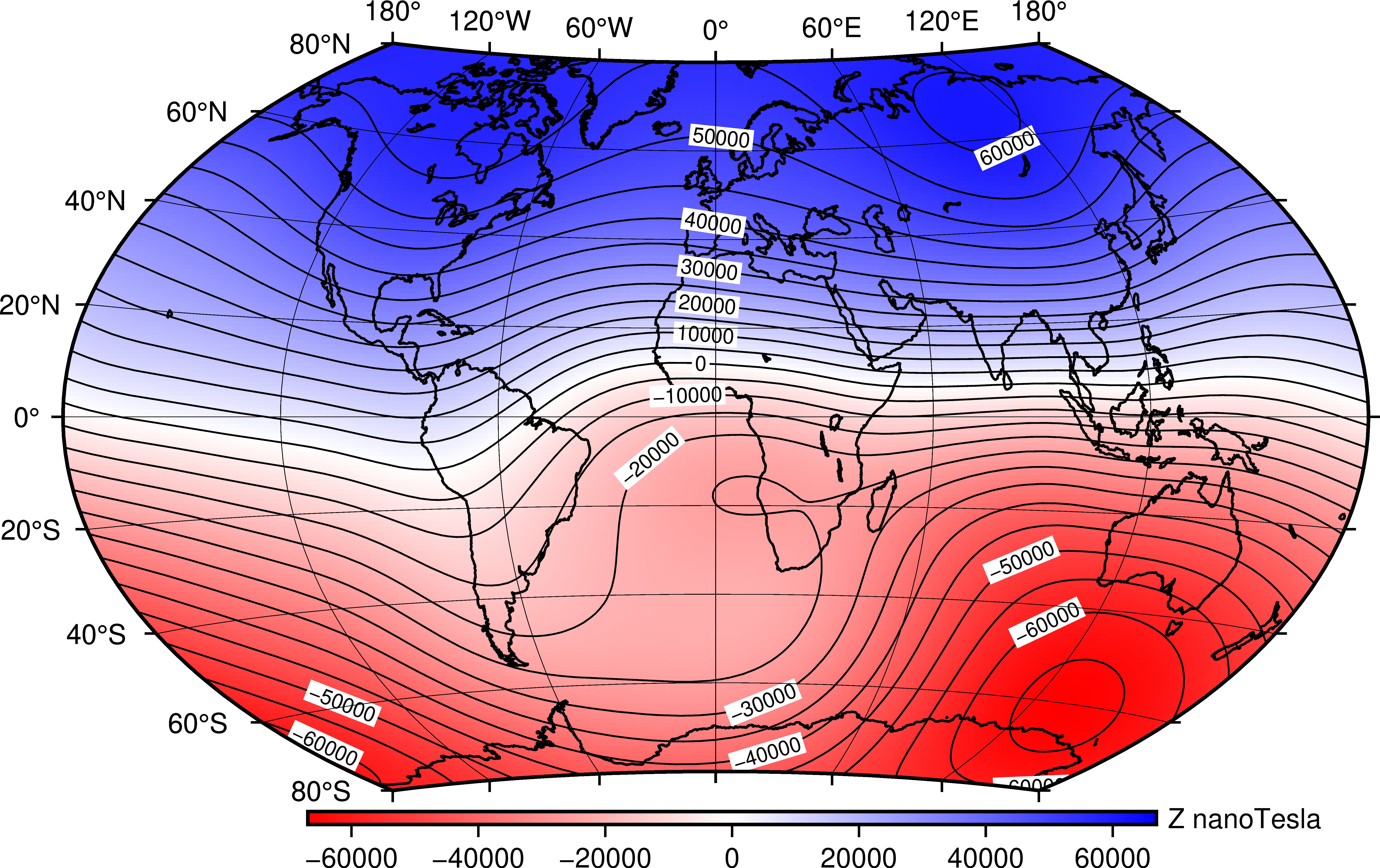
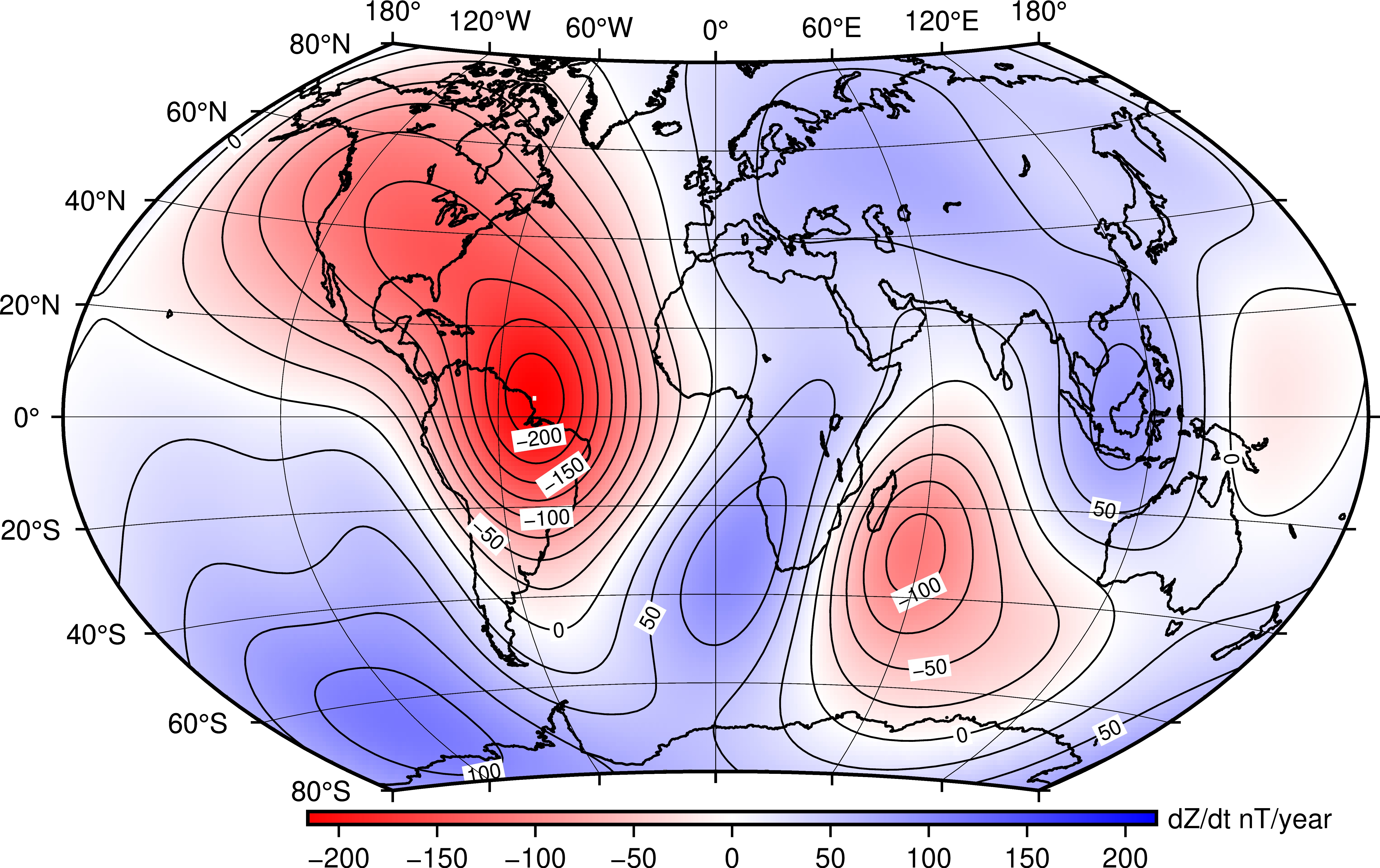
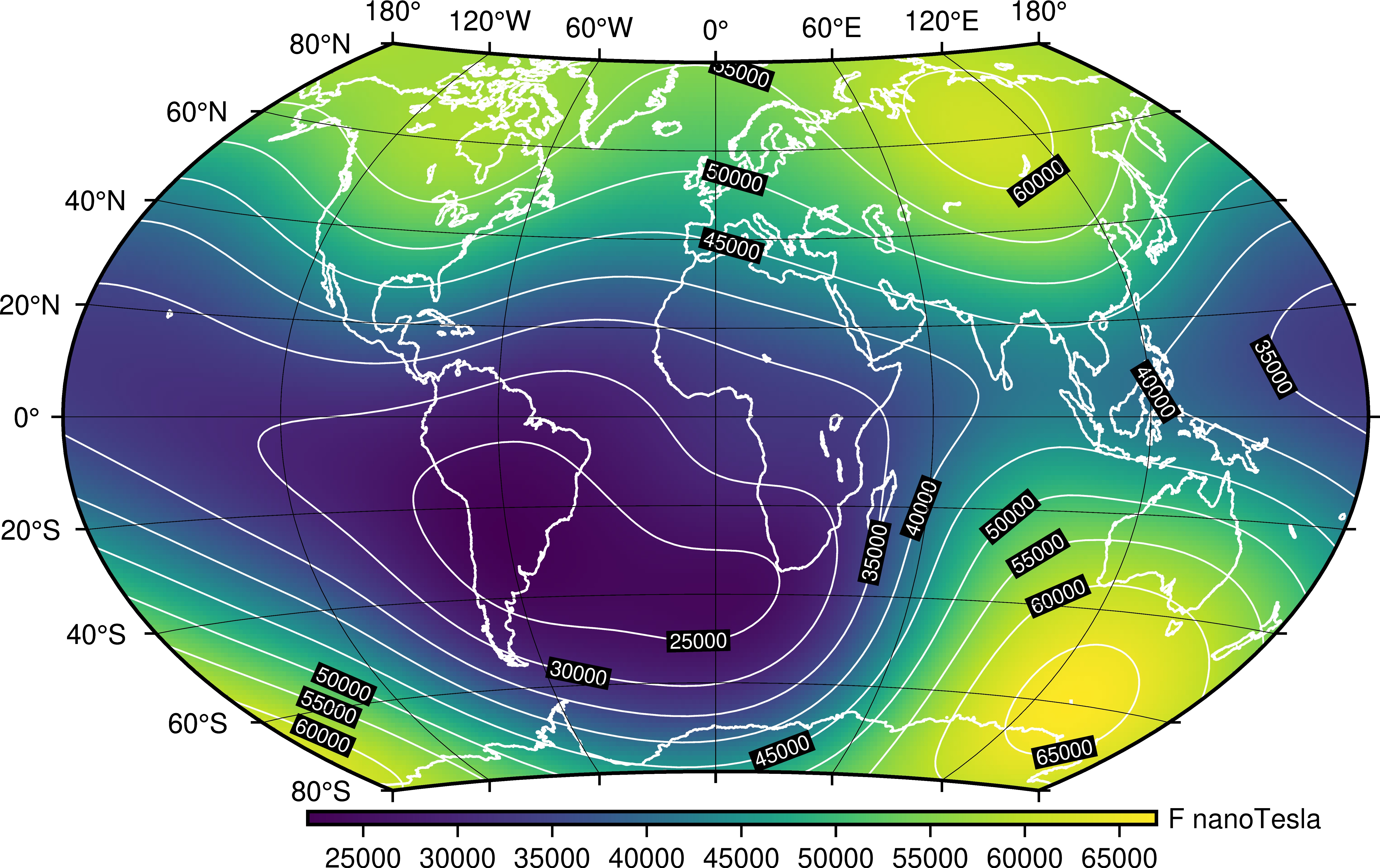
At the Earth's surface the main field can be approximated by a dipole placed at the Earth's centre and tilted to the axis of rotation by about 10�. However, significant deviations from a dipole field exist. Figures 2-11 show maps of declination, inclination, horizontal intensity, vertical intensity and total intensity at 2020.0, and their predicted secular variations for the period 2020.0 to 2025.0, derived from the 13th Generation IGRF model.
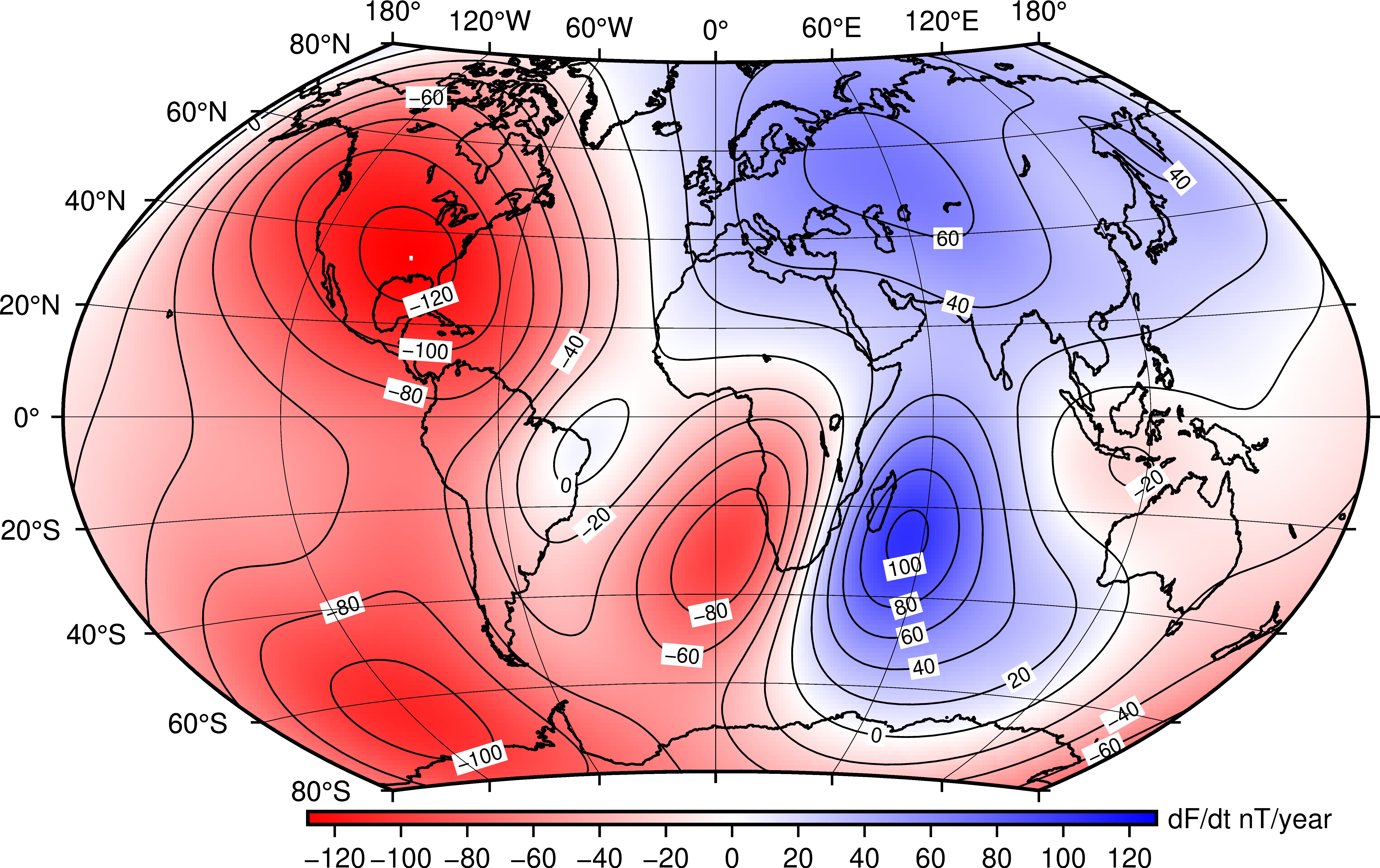
Back to the top of the page
3.3 Westward drift
Using direct observations of the magnetic field over the past 400 years, the pattern of declination seen at the Earth's surface appears to be moving slowly westwards. This is particularly apparent in the Atlantic hemisphere at mid- and equatorial latitudes. This may be related to the motion of fluid at the core surface slowly westwards, dragging with it the magnetic field.
Back to the top of the page
3.4 Geomagnetic jerks
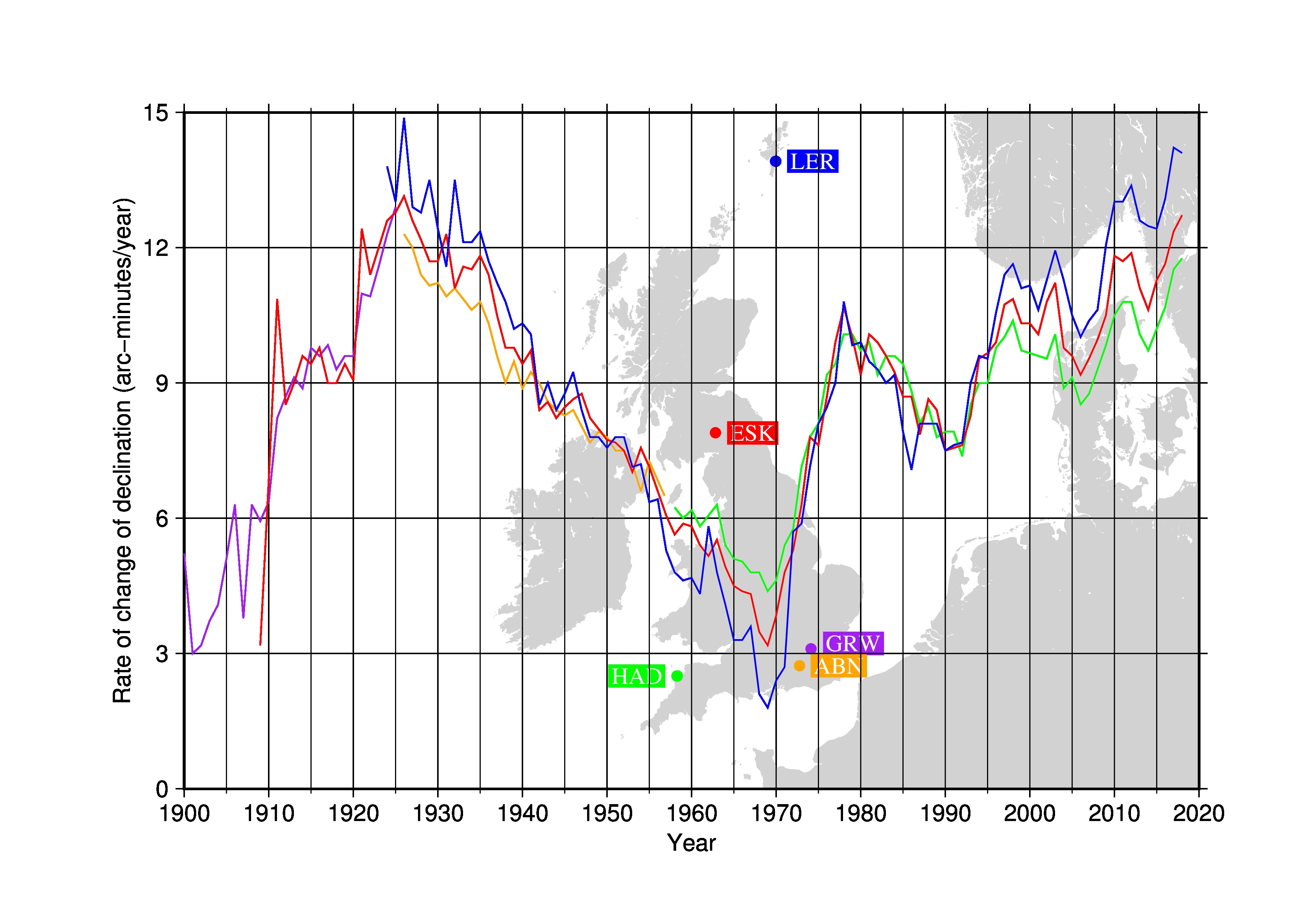
The rate of change of declination at Lerwick, Eskdalemuir and Greenwich-Abinger-Hartland observatory series in the UK is shown in Figure 12. It can be seen from this plot that there have been a number of changes in the general trend of secular variation in the past, in particular at about 1925, 1969, 1978 and 1992. These sudden changes are known as jerks or impulses and, at the present time, are not well understood and are certainly not predictable. Some researchers have found evidence for a correlation with length-of-day changes.
Back to the top of the page
3.5 Crustal magnetic field
The field arising from magnetic materials in the Earth's crust varies on all spatial scales and is often referred to as the anomaly field. A knowledge of the crustal magnetic field is often very valuable as a geophysical exploration tool for determining the local geology.
The anomalies seen at mid-ocean spreading ridges are of particular interest. At these locations molten mantle comes to the surface and solidifies to form new oceanic crust, preserving in it the strength and direction of the contemporary ambient magnetic field. As new material is extruded, the existing crust is pushed away on either side of the ridge, with the direction of the ambient magnetic field at time of formation frozen into it. Marine and aeromagnetic surveys reveal a series of stripes in the total intensity anomalies which run parallel to and symmetrically about the central ridge and these are interpreted as alternating blocks of normal and reversely magnetised oceanic crust. This discovery of a crude tape recorder of the Earth's magnetic field and its reversals was invaluable to the theory of plate tectonics developed in the 1960s.
Back to the top of the page
3.6 Field variations at quiet times
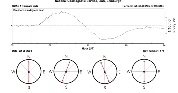
The geomagnetic field has a regular small variation with a fundamental period of 24 hours. This variation is easiest to observe during periods of low solar activity when large irregular disturbances are less frequent (see section 3.7 below). For this reason it is often referred to as the Solar quiet or Sq variation. Figure 13 shows the actual variation in declination recorded at Hartland observatory on June 22nd, 2004. This graph is typical of the smooth Sq variation seen at this latitude. Below this is the variation in a compass needle at Hartland over the same period. In reality, this type of variation in the geomagnetic field would affect the direction of a compass needle by no more than a few tenths of a degree. Inclination varies by less than a tenth of a degree and the total intensity of the magnetic field is perturbed by only a few tens of nT, which represents about 0.1% of the Earth's magnetic field strength at Hartland. Although these effects are very small, they can be of interest to those who use measurements of the Earth's magnetic field as a tool for very precise navigation (see sections 4.1 and 4.2 below).
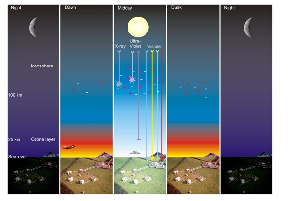
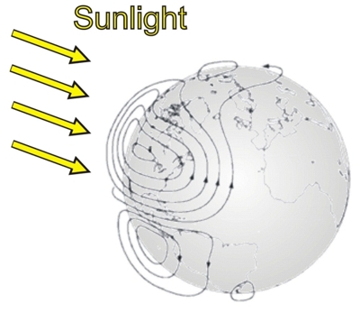
This regular fluctuation is caused by electrical currents high in the ionosphere, a region above about 100 km altitude. All currents, like those in wires, can only flow in materials that conduct. The copper used in wires conducts very well but the air is a poor conductor. However, in the ionosphere high energy ultra-violet rays and X-rays from the Sun displace electrons from (or ionise) the neutral (uncharged) molecules in the air to produce positive and negatively charged particles (see Figure 14, '+' and '-' represent the charged particles). These charges allow the air to conduct. At any point on Earth, the Sun is at its most intense around midday and is therefore generating the most charges in the ionosphere overhead, which allows the air to conduct better. After dusk, in the absence of ionising radiation, the charges begin to recombine into neutral molecules again and so the ability for the air to conduct is reduced. This cycle is repeated each day.
The sunlight not only makes the air conduct, it also heats it causing
winds. These winds combine with the tidal winds caused
by the gravitational pull of the Sun and Moon and the resulting thermo-tidal winds drive the ionospheric
dynamo. This dynamo generates currents as the conducting ionosphere
is driven through the Earth's magnetic field. These current systems
form two closed loops: an anti-clockwise vortex in the northern hemisphere
and a clockwise vortex in the southern hemisphere, like those shown
in Figure 15. Because it is solar radiation that produces the charges
that in turn let the atmosphere conduct, the currents remain predominantly
on the sunlit side of the Earth. It is these currents that produce the
daily magnetic field fluctuations as the Earth rotates beneath, which
explains why the magnetic field varies throughout the day. The shape,
size and location of these vortices also explain why the Sq variation
depends on latitude. As the amount of solar radiation falling upon the
northern and southern hemispheres varies with the seasons and solar
cycle, the Sq variation also varies.
Back to the top of the page
3.7 Field variations at disturbed times
As well as the regular daily variation the Earth's magnetic field also exhibits irregular disturbances, and when these are large they are called magnetic storms. These disturbances are caused by interaction of the solar wind, and disturbances therein, with the Earth's magnetic field. The solar wind is a stream of charged particles continuously emitted by the Sun and its pressure on the Earth's magnetic field creates a bounded comet-shaped region surrounding the Earth called the magnetosphere. When there is a disturbance in the solar wind the current systems existing within the magnetosphere are enhanced and cause magnetic disturbances and storms. Figure 16 shows a schematic picture of the solar wind and the Earth's magnetosphere.
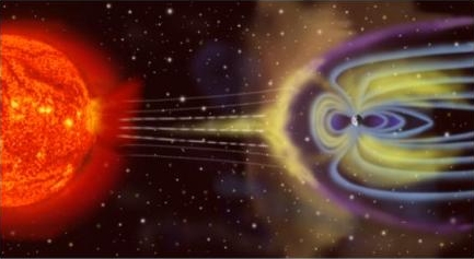
The amplitude of magnetic disturbances is larger at high latitudes because of the presence of the oval bands of enhanced currents around each geomagnetic pole called auroral electrojets. Some charged particles get trapped at the boundary of the magnetosphere and, in the polar regions, are accelerated along the direction of the magnetic field towards the atmosphere and finally colliding with oxygen and nitrogen molecules. These collisions result in sometimes spectacular emissions of mainly red and green light known as aurora borealis at northern latitudes and aurora australis at southern latitudes.
The prevailing conditions in the solar-terrestrial environment which are a consequence of the emission of charged particles from the Sun and their interaction with the Earth's magnetic field, is called space weather. There is presently some considerable interest in forecasting space weather and data from satellites observing the Sun and the solar wind are extremely valuable for this.
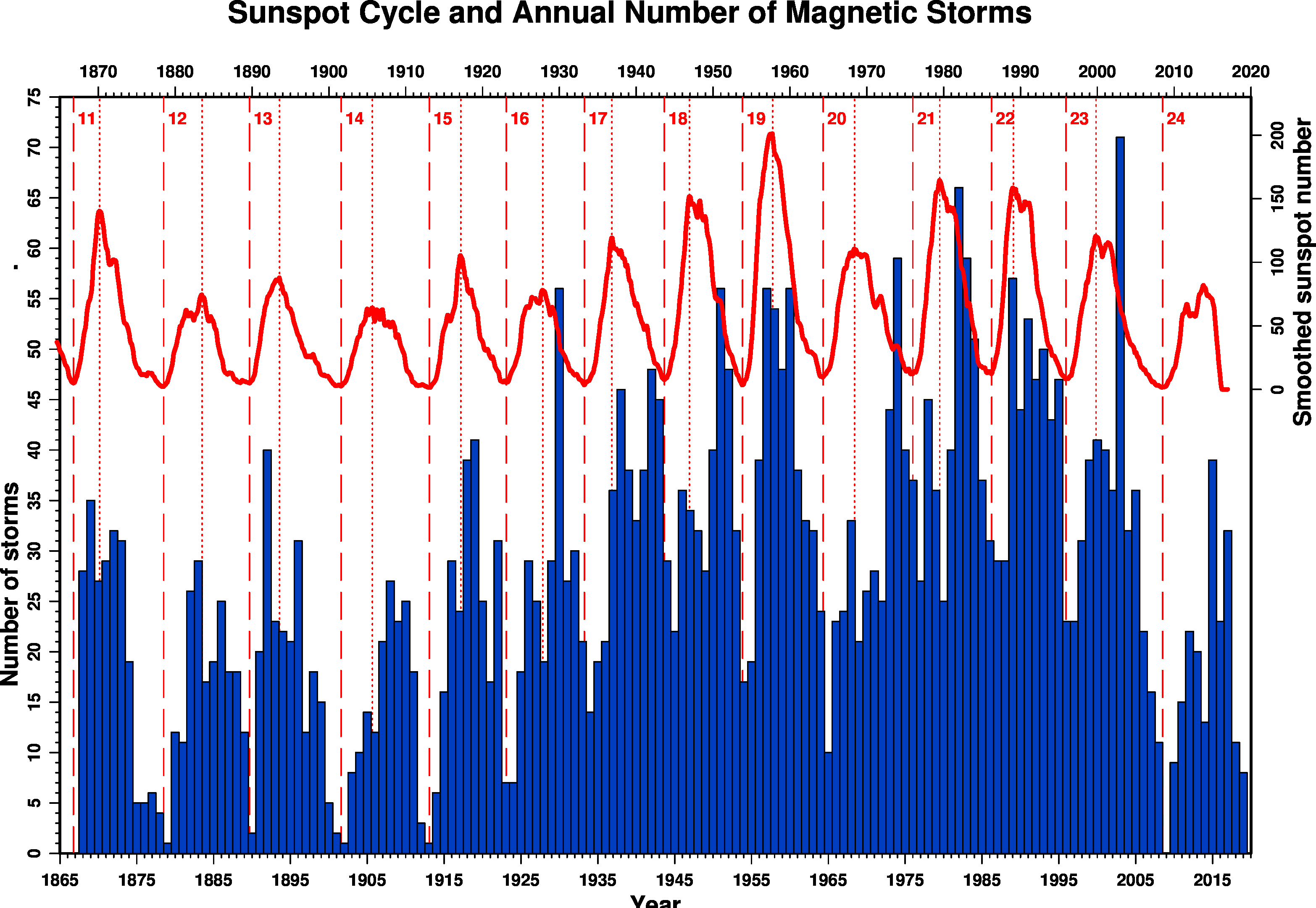
Although irregular, magnetic disturbances exhibit some patterns in their frequency of occurence. The main pattern is the correlation with the 11-year solar cycle and Figure 17 shows the number of magnetic storms per year, from 1868 to present and the corresponding number of sunspots. Another important pattern is the 27-day recurrence of some storms related to the 27-day rotation of the Sun as seen from Earth.
Back to the top of the page
4 The Earth's magnetic field as both a tool and a hazard in the modern world
4.1 Navigation
The earliest writings about compass navigation are credited to the Chinese and date from 11th century A.D. There is evidence of compasses being used in Europe about 100 years later but the first observations of declination were not recorded until the 16th century. In 1700 the first magnetic chart, covering the Atlantic Ocean, was produced by Halley.
Contemporary values of declination, or for some maps the difference between grid north and magnetic north (grid magnetic angle), are depicted on the majority of modern sea charts, topographic maps and aeronautical charts. These values must be kept up-to-date by regular revision of the models from which they are derived. This is an example of the Earth's magnetic field being a tool.
Back to the top of the page
4.2 Directional drilling
A specialist form of navigation is directional drilling in the petroleum industry. There are two main methods of navigation available for drilling deviated wells towards often small targets in the oil reservoirs. One method makes use of gyro tools but this can be expensive. The other method makes use of magnetic tools. As accuracy is critical for economic reasons and to avoid well collisions, the accuracy requirements on the Earth's magnetic field values, used to correct the direction of the well from magnetic bearings to true bearings, are typically 0.1� in direction and 50 nT in total intensity. To attain these accuracies account must be taken of the crustal field, daily variations and magnetic storms. This application is an example of the Earth's magnetic field being a tool in the modern world but it can also be a hazard if no account is taken of these other sources.
Back to the top of the page
4.3 Geomagnetically induced currents
The most severe magnetic storm in recent times occurred in March 1989 and this had a number of serious impacts on technological systems by generating damaging geomagnetically induced currents. In particular, the power transmission system in Quebec, Canada, was shut down for over 9 hours. Other effects such as increased corrosion in pipelines are also likely. This is an example of the Earth's magnetic field being a hazard in the modern world.
Back to the top of the page
4.4 Satellite operations
When a magnetic storm is underway the Earth's atmosphere expands because of heating, and increases the atmospheric drag on satellites at altitudes below about 1000 km. The orbit of the satellite can be changed and sometimes expensive manoeuvres must be made to compensate. Other effects on satellites are caused by radiation hits which can interfere with onboard computers. The prediction of magnetic activity, as a monitor of conditions at satellite altitude, is therefore of great interest to satellite operators. This is another example of the Earth's magnetic field being a hazard in the modern world.
Back to the top of the page
4.5 Exploration geophysics
Magnetic field, usually total intensity, traverses and surveys over an area can aid understanding of the underlying geology and in the case of iron ore deposits, can indicate very clearly their locations. This is an example of the Earth's magnetic field being a tool but it may turn into a hazard, especially at high latitudes, if care is not taken to remove the daily variations and magnetic storm effects from the data before interpretation.
Back to the top of the page
Bibliography
Campbell, W. H., 2003. Introduction to Geomagnetic Fields (2nd Ed). Cambridge University Press. [This book is an introduction to geomagnetism suitable for those who are not familiar with the field, with an emphasis on external fields.]
Christensen, U. R., A. Balogh, D. Breuer, K.-H. Glassmeier (Eds), 2010. Space Science Reviews Vol 152, 1-4: Planetary Magnetism. [Collection of articles suitable for researchers in planetary magnetic fields.]
Gubbins, D. and E. Herrero-Bervera (Eds), 2007. Encyclopedia of Geomagnetism. Springer. [Collection of more than 300 articles with emphasis on core and crustal fields and paleomagnetism.]
Hulot, G., A. Balogh, U. R. Christensen, C. Constable, M. Mandea, N. Olsen (Eds), 2010. Space Science Reviews Vol 155, 1-4: Terrestrial Magnetism. [Collection of articles suitable for researchers in geomagnetism.]
Jankowski, J., and C. Sucksdorff, 1996. IAGA Guide for Magnetic Measurements and Observatory Practice. International Association of Geomagnetism and Aeronomy. [This book describes magnetic observatory instrumentation and procedures, and is suitable for those setting up or running an observatory and using observatory data.]
Jacobs, J. A. (Ed), 1987. Geomagnetism Volumes 1, 2 and 3. Academic Press. [Volume 1: history of geomagnetism, instrumentation, overviews of main and crustal fields. Volume 2: origins of the Earth's magnetic field and that of the moon and other planets. Volume 3: rock magnetism, palaeomagnetism and the ancient magnetic field behaviour, conductivity structure of the Earth, indices of geomagnetic activity, magnetic field characteristics during solar quiet conditions.]
Jacobs, J. A. (Ed), 1991. Geomagnetism Volume 4. Academic Press. [This volume covers the solar-terrestrial environment including the solar wind, the Earth's magnetosphere, magnetopause, magnetotail, ionosphere, pulsations, plasma waves, magnetospheric storms and sub-storms, auroras.]
Kono, M. (Ed), 2009. Geomagnetism: Treatise on Geophysics Vol. 5. Elsevier. [Collection of articles with emphasis on core and crustal fields and paleomagnetism.]
Mandea, M. and M. Korte (Eds), 2011. Geomagnetic Observations and Models (IAGA Special Sopron Series Vol 5), Springer. [Collection of articles suitable for researchers and scientists in geophysics and geomagnetism.]
Merrill, R. T., M. W. McElhinny and P. L. McFadden, 1996. The Magnetic Field of the Earth. Academic Press. [This book is an introduction to geomagnetism suitable for those who are not familiar with the field, with an emphasis on core and crustal fields and palaeomagnetism.]
Parkinson, W. D., 1983. Introduction to Geomagnetism. Scottish Academic Press. [This book is an introduction to geomagnetism suitable for those who are not familiar with the field.]
Back to the top of the page

